🔍 Stencil Aperture Design: A Key to SMT Success In Surface Mount Technology (SMT), the stencil aperture directly influences solder paste deposition — and ultimately, the reliability of your PCB assembly. So, what exactly is a stencil aperture? 👉 It's the opening in the stencil foil that allows solder paste to be printed onto PCB pads. ⚙️ Common Types of Stencil Apertures 🔹 Square / Rectangular – Most common, ideal for chips (resistors, capacitors) – Ensures uniform paste volume 🔹 Circular – Used for vias or special pad designs – Offers controlled paste release 🔹 Home Plate – Helps reduce tombstoning defects – Great for chip components 🔹 Inverted Home Plate – Minimizes solder balling – Improves paste distribution during reflow 🔹 Window Pane – Best for large pads (e.g., QFN, thermal pads) – Reduces excess solder and voiding 🔹 Step (Step-up / Step-down) – Varies paste thickness for mixed component sizes – Balances fine-pitch and large-component printing ✅ Why Aperture Design Matters ✔ Controls solder volume with precision ✔ Reduces defects like tombstoning, bridging & voiding ✔ Boosts yield and long-term reliability ✔ Drives consistent printing performance 💡 Pro Tip Optimize your stencil design based on component types, PCB layout, and process capability. There’s no universal solution — only the right fit for your application. #SMT #ElectronicsManufacturing #PCBAssembly #StencilDesign #SolderPaste #QualityEngineering #PCBDesign

Boost your Altium Designer efficiency by 50% with these 10 hidden gems ⚡ As PCB designers, we all know the feeling: hours lost navigating menus and repeating manual steps. The real productivity leap doesn’t come from clicking faster — it comes from knowing the right shortcuts. After years of refining my workflow, here are 10 Altium hacks that made the biggest difference: Find Similar Objects (FSO) – Right‑click → Find Similar → batch‑edit 100 components in seconds. Smart Alignment – Use A shortcuts (AL, AT, AD) to snap components into place instantly. Single Layer Mode (Shift+S) – Eliminate visual clutter and focus only on the layer you’re working on. Routing Modes (Shift+R) – Switch between Push and Walkaround mid‑trace without restarting. Quick Via / Layer Switch – Use + / - on the numpad while routing to auto‑place vias. Length Tuning (TR) – Create accordion traces like a pro; hit Tab to tweak settings on the fly. 3D Navigation – 3 to enter 3D view, Shift+Right‑click to rotate, 0 to reset. Mirroring (X / Y) – Flip components instantly while dragging. Selection Filter – Lock onto Polygons or Text so you only grab what you need. Paste Special (E+A) – Duplicate complex layouts while preserving net connectivity. Which of these do you already use — and what’s your #1 Altium time‑saver? Let me know in the comments 👇 #PCBDesign #AltiumDesigner #EngineeringProductivity #AltiumTips

Oscilloscopes can play like this The melody that beats, the radio frequence that dances.

5 Common PCB Signal Termination Methods – and when to actually use them 🚀 Signal termination is often an afterthought. But in high-speed PCB design, it directly impacts signal integrity, EMI, and production stability. Here’s a practical breakdown of 5 termination methods – and where each makes sense. 👇 1️⃣ Point‑to‑Point (No Termination) One driver, one receiver. Works for short traces & slow edge rates. ⚠️ Risk: impedance mismatches → reflections & ringing. ✅ Use for: low‑speed signals, short traces, tolerant logic. 2️⃣ Source (Series) Termination A resistor near the driver matches trace impedance. ✅ Low power, simple, common for CMOS & clocks. ❌ Not for multi‑drop buses. 3️⃣ Parallel Termination Resistor at the receiver matches trace Z. ✅ Clean waveform, great for high‑speed signals. ⚠️ Trade‑off: constant DC power draw – avoid in low‑power designs. 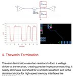4️⃣ Thevenin Termination Two resistors form a divider – matches impedance + sets logic bias. ✅ Good SI with DC level control. ✅ Common in high‑speed memory (DDR) – often as on‑die termination. 5️⃣ RC Termination Resistor + capacitor absorbs AC reflections, blocks DC. ✅ Lower power than parallel, reduces overshoot. ❌ Slows edges, limited bandwidth. ✅ Good for moderate‑speed control / enable signals. 📌 DFM Reality Check From a manufacturing standpoint: Termination resistors must be placed close to source or load – otherwise they lose effectiveness. Inconsistent placement = board‑to‑board SI variation. Extra components affect BOM cost, placement yield, and rework risk. A termination scheme that only works in simulation but is sensitive to placement tolerance is not production‑robust. Signal integrity choices must consider layout feasibility & assembly repeatability – not just clean waveforms. “Good design is buildable design.” What’s your go‑to termination method for high‑speed interfaces? Let’s discuss in the comments. 👇 #PCBDesign #SignalIntegrity #HardwareEngineering #DFM #ElectronicsManufacturing

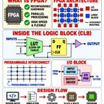
FPGA (Field Programmable Gate Array) is a reconfigurable semiconductor device that allows engineers to create custom digital circuits after manufacturing. Unlike a conventional processor that executes instructions sequentially, an FPGA can perform multiple hardware operations simultaneously. An FPGA contains thousands of configurable logic blocks (CLBs), programmable interconnections, and input/output blocks. Each logic block typically contains Look-Up Tables (LUTs) and Flip-Flops (FFs). LUTs implement combinational logic functions, while flip-flops store data and support sequential operations. Programmable routing connects these blocks to form complex digital systems. The FPGA design process begins with hardware description languages such as Verilog or VHDL. Engineers simulate the design, synthesize the logic, perform placement and routing, generate a configuration bitstream, and program the FPGA. FPGAs are widely used in wireless communication, radar, aerospace, industrial automation, automotive electronics, image processing, and cybersecurity. Their major advantages include parallel processing, low latency, hardware flexibility, and high-speed signal processing.

🛡️ Why ESD Protection Doesn’t Stop at the Chip Many modern ICs include internal ESD protection – but that’s only part of the story. 📄 Datasheet ratings typically show: ▪️ HBM: 2–4 kV ▪️ CDM: 250–500 V ⚠️ System-level requirements (IEC 61000-4-2) can demand: ▪️ 8 kV contact discharge ▪️ 15 kV air discharge That’s why external ESD protection is still essential – especially for connectors and user-accessible interfaces. Let’s break down a few common protection circuits 👇 🟡 1. TVS Diodes (still the workhorse) Normal operation → open circuit During ESD → avalanche breakdown, surge current diverted to GND ✅ Common applications: USB, HDMI, Ethernet, GPIO lines, power inputs 🔑 For high-speed interfaces: choose low-capacitance TVS (<0.5 pF) to preserve signal integrity. 🟡 2. Rail Clamp Diodes A simple but effective structure using diodes connected to power rails: Voltage > VCC → upper diode conducts, clamps Voltage < GND → lower diode conducts, clamps negative transients ✅ Ideal for MCU GPIO protection and low-speed interfaces. 🟡 3. Unidirectional vs. Bidirectional TVS Unidirectional → DC power rails (clamps positive transients) Bidirectional → differential or AC signals (clamps both polarities) Selection depends on signal type, operating voltage, and interface bandwidth. 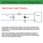🟡 4. High-Energy Surge Protection (industrial / telecom) Additional devices come into play: 🔹 GDTs, MOVs, multilayer varistors, polymer suppressors 🔁 Common combo: GDT + TVS GDT handles large surge energy TVS provides fast voltage clamping Layered protection = robust designs in harsh environments. 🎯 The takeaway Internal ESD structures protect chips during manufacturing & handling. But system-level ESD protection must be designed at the board level – especially for external interfaces. 👉 In my next post: PCB layout rules for effective ESD protection. 💬 Have you ever faced ESD failures at the system level despite “protected” ICs? Let me know in the comments. #ESD #CircuitDesign #HardwareEngineering #PCBDesign #EmbeddedSystems

MOAR Sparkle Motion testing - built-in I2S mic

Voltage Regulator Quick Reference: AMS1117 & LM2596S 🔧 Whether you're troubleshooting a repair or selecting a part for your next project, this quick guide breaks down two of the most common voltage regulator families—their output variants and pin configurations. 🔹 AMS1117 Linear Regulators Common fixed-output variants: • AMS1117-5.0 → 5.0V • AMS1117-3.3 → 3.3V • AMS1117-1.8 → 1.8V • AMS1117-1.5 → 1.5V • AMS1117-1.2 → 1.2V Pinout (1–3): GND · OUT · IN 🔹 LM2596S Switching Regulators Fixed-output variants: • LM2596S-3.3 → 3.3V • LM2596S-5.0 → 5.0V • LM2596S-12 → 12V Pin labels: V-IN V-OUT GND Feedback ON/OFF Keep this handy when identifying regulator markings or reviewing pin labels on the bench. ⚠️ Always verify the exact package pinout against the manufacturer's datasheet before making circuit connections. Created or enhanced with AI tools for creative and educational purposes. #VoltageRegulator #Electronics #SMD #IC #Tech #Engineering

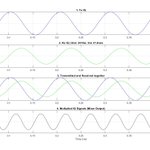
Deciphering the "Beat": The Physics of IQ Mixing in Doppler Radar 📡⚡ In RF engineering and Electronic Warfare, a target's velocity isn't just a number — it's a frequency shift hidden inside a complex signal. I recently ran a series of simulations at 9.65 GHz to visualize how radar "sees" motion through IQ signal multiplication (mixing). The results (frames Velocity1–Velocity4) offer a clear window into the physics of Doppler processing. 👇 Here's what's happening: 1. The Phase-Coherent Baseline Every detection starts with the Tx Reference (blue). By comparing it to the Rx Echo (green), we see the time-of-flight delay. As the distance shifts from 2410 m to 5000 m, the phase lag changes — the very foundation of pulse-Doppler processing. 2. Non‑Linear Magic: Signal Multiplication Multiplying transmitted and received IQ signals isn't just "adding" waves — it's hardware mixing. The result produces a difference frequency: the Doppler shift, or the "beat" frequency we actually care about. 3. Linear Scaling of the Doppler Shift The simulation perfectly validates the Doppler equation: fd = 2·v·fc / c At 10.0 m/s → 0.64 kHz beat At 20.0 m/s → 1.29 kHz beat (doubles as expected) At 41.9 m/s → 2.69 kHz beat Linear, undeniable, and beautifully predictable. 4. Why This Matters for EW & Counter‑Drone Systems In high‑clutter environments, static objects (buildings, trees) produce a Doppler shift of 0 Hz. By mixing the signals and applying a low‑pass filter (LPF) to the mixer output, we effectively "blind" the radar to anything not moving. That means we can isolate a fast‑moving drone or vehicle — even when its radar cross‑section (RCS) is tiny compared to the background. Physics + signal processing + real‑world EW impact. That's the kind of engineering worth diving into. Have you used IQ mixing for low‑RCS detection or counter‑UAS applications? Let's discuss below. 👇 #RadarEngineering #SignalProcessing #MATLAB #ElectronicWarfare #RFDesign #DopplerEffect #DeepTech #ElectricalEngineering #DigitalSignalProcessing #DSP #RF #RFEngineering #CommunicationEngineering #WirelessCommunications #EngineeringLife #FrequencyDomain #TimeDomain #ActiveRadar #Radar

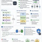
🚀 Bootloader in Embedded Systems – The First Code That Runs When an embedded device powers on, your application isn't the first to run. A Bootloader takes control first. It initializes the system and decides what happens next. Let’s break it down 👇 🧠 What is a Bootloader? A small program stored in non-volatile memory that runs immediately after reset or power‑up. Its job → prepare the hardware, then launch the main firmware. ⚙️ What a Bootloader Does ✅ Initializes hardware peripherals  • Clock & memory setup  • GPIO / UART configuration ✅ Verifies firmware integrity  • Checksum / CRC validation ✅ Loads the main application  • Jumps to application code ✅ Supports firmware updates  • UART, USB, CAN, OTA 🔄 Typical Boot Flow Power ON → Bootloader starts → Hardware init → Firmware verification → Jump to application 💡 Types of Bootloaders 🔹 Primary – Stored in ROM/internal flash, runs immediately after reset 🔹 Secondary – Handles advanced tasks like firmware updates 📌 Why Bootloaders Matter • Secure firmware updates • Recovery from corrupted firmware • Remote upgrade capability • Essential for production devices 💻 Code Example (Jump to Application) c #define APP_START_ADDRESS 0x08004000 typedef void (*AppFunction)(void); void jump_to_application() { AppFunction app_entry; app_entry = (AppFunction)(*((volatile uint32_t*)(APP_START_ADDRESS + 4))); __set_MSP(*(volatile uint32_t*)APP_START_ADDRESS); app_entry(); } ⚠️ Common Challenges • Secure boot implementation • Handling flash corruption • Memory partitioning • Update failure recovery 🎯 Key Insight A bootloader is the foundation of embedded startup – enabling secure boot, reliable updates, and robust system initialization. 💬 What’s your experience with bootloaders? Ever faced a tricky update failure? Let’s discuss below. #EmbeddedSystems #Bootloader #FirmwareDevelopment #EmbeddedEngineering #IoT

🚀 The Evolution of Radar Arrays: From Passive to Digital Dominance Radar technology has come a long way—from rigid analog architectures to agile, software-defined systems that are redefining sensing and surveillance. Let’s break down the journey: 🔹 Passive Array Centralized high-power amplifier + analog beamforming. ✅ Robust ❌ Limited flexibility and scalability 🔹 Active Array (AESA) Distributed T/R modules enable electronic beam steering, improved reliability, and multi-target tracking. ✅ Major leap in performance and resilience 🔹 Digital Array Full digital beamforming with per-element A/D conversion + DDS. ✅ Simultaneous multi-beam operation ✅ Adaptive waveform control ✅ Enhanced ECCM ✅ Superior target discrimination 💡 Key takeaway: This isn’t just an upgrade—it’s a paradigm shift. Digital arrays bring software-defined flexibility, making radar systems smarter, faster, and mission-ready for complex operational environments. 📡 From legacy systems to cutting-edge architectures, radar continues to drive innovation across defense, aerospace, and beyond. What stage of this evolution are you most excited about? Let’s discuss below 👇 #Radar #AESA #DigitalBeamforming #DefenseTechnology #Aerospace #SystemsEngineering #Innovation #SignalProcessing

Understanding Impedance Matching in Antenna Design 📡 Impedance matching is a fundamental concept in RF and antenna engineering. It ensures maximum power transfer from the transmission line to the antenna—without it, even the best antenna structure can underperform. 🔹 Why 50Ω? For optimal performance, an antenna’s input impedance should be as close as possible to the standard reference impedance of 50Ω. 🔹 Matching at a glance: Z ≈ 50Ω → Ideal matching Small mismatch → Acceptable performance Large mismatch → Poor performance In practice, perfect matching is rarely achieved. Mismatches cause signal reflections, which are measured using parameters like return loss and VSWR. When reflection occurs, part of the signal never gets transmitted, leading to: ❌ Power loss ❌ Lower efficiency ❌ Reduced overall system performance That’s why engineers focus heavily on matching antenna impedance to the transmission line. 🔧 In my work with CST Studio Suite, I optimize matching by tuning parameters such as feed position, dimensions, and material properties. Getting the antenna impedance and transmission line to work in harmony is always a top priority. #AntennaDesign #RFEngineering #MicrowaveEngineering #WirelessCommunication #EEE #Research #CSTStudio #Engineering

RO4350B: Built for RF Design Explore Rogers RO4350B high-frequency PCB material: a glass-reinforced hydrocarbon/ceramic laminate for RF and microwave circuits. Start with the frequency range, loss budget and fabrication requirements before selecting your stackup. #RO4350B #RogersPCB #RFDesign #PCBDesign #RAYPCB

How to Properly Measure Capacitance on a Circuit Board #Multimeter Usage #How to Measure Capacitance

From simple current-to-voltage conversion to the heart of high-speed optical links – the evolution of the Transimpedance Amplifier (TIA) 📡⚡ TIAs are the unsung front-end heroes of optical receivers, converting tiny photocurrent from a photodiode into usable voltage. What started as a basic interface has become a critical enabler of performance and efficiency in modern optical systems. 🔹 1970s – The beginning Early TIAs used op-amp based conversion, sufficient for low data rates. But as speeds increased, the RC time constant at the input (dominated by photodiode capacitance) became a bottleneck. 🔹 2000s – Entering the RF domain Low-input-impedance topologies (common gate, regulated cascode) emerged. Inductive peaking, multi-stage amps, and impedance matching balanced gain, bandwidth, and noise. The feedback resistor became a key tradeoff node. 🔹 2010s – PAM4 and linearity Multi-level signaling made distortion a major concern. TIAs began integrating equalization, programmable gain, and adaptive biasing to maintain linearity. 🔹 Device & packaging realities Higher photodiode responsivity = higher capacitance = lower bandwidth. CMOS offers integration; SiGe and InP deliver speed. Packaging parasitics now dictate high-frequency performance. 🔹 Today – 800G / 1.6T era Photonic integration and co-packaged optics reduce parasitics. With AI data centers pushing to offload DSP, more functionality is moving into the analog front end – TIAs are absorbing equalization, gain control, and calibration. 🔜 Looking ahead Optical I/O will move closer to ASICs. Expect ultra-low-power designs, adaptive analog front ends, and heterogeneous integration to define next-gen systems. From a simple converter to a core system component – the TIA continues to evolve, shaping the future of high-speed, energy-efficient communication. What trends do you see shaping analog front-end design in the next 5 years? Let me know below 👇 #TransimpedanceAmplifier #OpticalCommunications #HighSpeedDesign #Semiconductors #PAM4 #CoPackagedOptics #AnalogDesign

How the flying probe test works on circuit boards

7 Tips for Routing Controlled Impedance Traces 🧵⚡ Controlled impedance routing is one of the most critical aspects of high-speed PCB design. Small layout mistakes can cause signal integrity problems, reflections, EMI, and unstable communication. Here are 7 practical tips I always follow when routing controlled impedance traces: ✅ Keep differential pairs symmetrical and parallel ✅ Use uniform via placement to avoid plane discontinuities ✅ Apply proper length matching techniques ✅ Avoid routing over split planes ✅ Keep differential pairs on the same layer whenever possible ✅ Maintain symmetry around coupling capacitors ✅ Add stitching vias close to signal transitions Good PCB design isn’t just about making connections — it’s about ensuring signal quality and reliability across the entire system. Which of these rules do you consider the most important in your PCB layouts? 👇 #PCBDesign #HardwareDesign #ElectronicsEngineering #AltiumDesigner #SignalIntegrity #HighSpeedDesign #EmbeddedSystems #Electronics #PCBlayout #Engineering

Analog Circuit Design Interview Question Consider a 5-transistor OTA. The DC voltage at the gate terminals of M1 and M2 is the same. M1 has 4 times the W/L ratio of M2. Derive the single-ended differential gain Ad = vout / vid = vout / (Vin1 - Vin2) in terms of transistor parameters and the biasing current. Will the biasing current be equally divided between M1 and M2 regardless of their W/L ratio, or will it depend on W/L? Share your answers and reasoning below. #AnalogCircuits #OTA #InterviewPrep #Engineering

IR Drop in Physical Design – The Silent Performance Killer ⚡ Your timing report looks clean. But if IR Drop isn’t managed, the chip can still fail in silicon. In VLSI Physical Design, power integrity is just as critical as timing closure. Let’s break it down 👇 What is IR Drop? A voltage drop caused by current flowing through the resistance of the power delivery network (PDN). 📐 Based on Ohm’s Law: V = I × R I = Current drawn by the circuit R = Resistance of metals / vias Types of IR Drop 🔹 Static IR Drop Due to average current flow. Depends on cell density and power grid strength. Seen during steady‑state operation. 🔹 Dynamic IR Drop Caused by switching activity. Sudden current spikes → voltage droop. Critical near clock edges and high‑switching blocks. Why IR Drop is Dangerous ❌ Slows down cells → timing violations ❌ Setup / hold failures ❌ Functional errors ❌ Increased leakage variability ❌ Chip failure in worst cases Root Causes Weak power grid (thin metals) High current density regions Poor via connectivity Long power routes Uneven cell placement How to Fix IR Drop 🛠️ ✅ Use wider metal layers for VDD/VSS ✅ Add more power stripes / straps ✅ Strengthen power rings ✅ Improve via stacking ✅ Optimize cell placement (reduce hotspots) ✅ Use decap cells for voltage stability Analysis Techniques 📊 Static IR Analysis → Average voltage drop 📈 Dynamic IR Analysis → Peak voltage droop Tools: RedHawk, Voltus, PrimeTime PX Key Insight Even a small voltage drop can: Increase delay Break timing Impact reliability Final Thought In Physical Design: Power Integrity = Timing Integrity Ignoring IR Drop is like building a highway without checking the fuel supply — eventually, everything stops. #VLSI #PhysicalDesign #IRDrop #PowerIntegrity #ASIC #Semiconductor #ChipDesign #VLSIDesign

High Frequency Oscillation #PS5 Grip Internal Trigger Structure #Mechanical Circuits