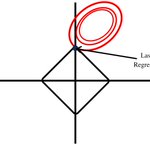
LASSO (Least Absolute Shrinkage and Selection Operator) is a regularization algorithm for linear regression that performs prediction and variable selection simultaneously. Given observations (xᵢ,yᵢ), the LASSO estimator solves β̂ = argminβ { (1/2n)∑ᵢ(yᵢ − xᵢᵀβ)² + λ‖β‖₁ }, where λ ≥ 0 controls the strength of regularization and ‖β‖₁ = ∑ⱼ|βⱼ| is the L₁ norm. Unlike ordinary least squares, the L₁ penalty can force some estimated coefficients exactly to zero, producing a sparse model. The geometric shape of the L₁ constraint explains this behavior: its corners make solutions more likely to lie on coordinate axes. LASSO therefore provides a principled approach to high-dimensional prediction when many candidate variables may be irrelevant. It is particularly important when p, the number of predictors, is comparable to or substantially larger than n, the sample size. LASSO has applications in statistical machine learning, including feature selection, high-dimensional regression, genomics, signal processing and compressed sensing. Its extensions—such as Elastic Net, Group LASSO and adaptive LASSO—allow different forms of structural sparsity. The method beautifully connects statistical regularization, convex optimization and the modern theory of high-dimensional inference.

Luis Martínez-Zoroa and His Contributions to PDE: Luis Martínez-Zoroa is a young mathematician working at the intersection of PDE, harmonic analysis and incompressible fluid dynamics, with a particular focus on singularity formation and loss of regularity. His work has addressed some of the most delicate questions surrounding Euler, Navier–Stokes and Surface Quasi-Geostrophic (SQG) equations. A central theme of his research is understanding how initially smooth solutions can lose regularity. With Diego Córdoba, he constructed global unique solutions of dissipative SQG that undergo instantaneous loss of regularity in the supercritical regime. They also established strong ill-posedness results for SQG in critical function spaces. His recent work has moved toward finite-time singularity formation in three-dimensional fluid equations. With Córdoba and Fan Zheng, he proved finite-time singularities for the 3D incompressible Euler equations through a novel blow-up mechanism. Even more recently, the same collaboration established finite-time blow-up for forced hypodissipative Navier–Stokes equations, showing that classical finite-energy solutions can become singular under fractional dissipation below a critical threshold. Together, these results form an important programme for understanding the fundamental question: Can nonlinear fluid equations evolve from smooth data to singular states in finite time? Martínez-Zoroa's work is particularly notable for developing rigorous mechanisms for regularity breakdown, ill-posedness and singularity formation—central themes in modern nonlinear PDE.

STATISTICS:

Optimal Transport for Network Comparison: Optimal Transport (OT) provides a principled way to compare networks by treating them as distributions of nodes, edges, features, or embeddings rather than comparing them only through graph-level statistics. Given two probability distributions μ and ν, OT seeks the cheapest way to transform μ into ν: W_c(μ,ν) = inf₍π∈Π(μ,ν)₎ 𝔼₍(x,y)∼π₎[c(x,y)], where c(x,y) is the cost of transporting mass from x to y and Π(μ,ν) is the set of couplings with marginals μ and ν. For networks, nodes can be represented by feature vectors, degrees, centralities, or learned embeddings. OT then finds a soft correspondence between nodes of two networks, making it useful even when the networks have different sizes or no obvious node-to-node alignment. A major advantage is that OT compares the geometry and distribution of network structure, rather than relying solely on handcrafted summary statistics. Entropic regularization, Wε(μ,ν) = minπ∈Π(μ,ν) ⟨π,C⟩ + ε∑ᵢⱼ πᵢⱼ(log πᵢⱼ−1), also makes computation substantially faster via Sinkhorn-type algorithms. In Statistics, OT enables distributional comparison, clustering and hypothesis testing for network populations. In ML, it supports graph matching, domain adaptation, graph representation learning and generative modeling. In AI, it can compare knowledge graphs, social networks, molecular graphs and neural representations. The key idea is simple: instead of asking whether two networks have the same nodes, ask how much “work” is required to transform the structure of one network into the other.

After all these while, we land up with this? 🤣🤣🤣

Hugo Duminil-Copin: Mathematics, Probability & AI Hugo Duminil-Copin is one of today’s leading mathematicians in probability and statistical physics, and a 2022 Fields Medallist. His work has transformed our understanding of phase transitions, percolation and interacting particle systems, particularly the Ising and Potts models. He developed powerful results on critical phenomena, sharp phase transitions and dependent percolation, connecting probability, combinatorics and mathematical physics. The Fields Medal recognized his work on longstanding problems concerning phase transitions, especially in dimensions 3 and 4. What makes his perspective especially interesting today is his view of AI and mathematics. In his article “Care for a little more AI?”, published August 30, he reflects on the growing role of AI in mathematical research. The interesting question is not simply whether AI can solve mathematics, but what happens when machines become increasingly capable of generating conjectures, finding patterns and assisting with proofs. Mathematics, however, is not merely about producing a correct answer: it is also about discovering why something is true, finding the right concepts, and communicating a proof that humans can understand. Duminil-Copin’s career offers a useful perspective: deep mathematics often emerges from identifying the right structure behind seemingly simple probabilistic questions. AI may become an extraordinary tool for exploring that structure—but the mathematician’s role in deciding which questions matter and why may remain fundamental. Article: proofsandprompts.com/2026/08…

Online Bayesian Learning Online Bayesian learning is the process of updating our beliefs about an unknown parameter or model as new data arrive sequentially. Instead of retraining from scratch, we maintain a posterior distribution and update it with each observation: Prior → New data → Posterior → Next prediction Why is it useful? • Statistics: sequential inference, Bayesian filtering, adaptive experiments & uncertainty quantification. • Machine Learning: online prediction, concept drift, Bayesian neural networks & personalized models. • Reinforcement Learning: uncertainty-aware exploration, Bayesian bandits, model-based RL & learning under partial information. The key advantage: you don't just learn a point estimate—you continuously learn a distribution over what you believe. That makes online Bayesian learning especially powerful when data arrive continuously and decisions must be made under uncertainty.

Generative Embedding Translation (GET): GET Better Medical Segmentation with 31% Fewer Trainable Parameters. Medical image segmentation is crucial for identifying tumors, lesions, organs, and other structures accurately, but existing approaches face a trade-off between accuracy and computational cost. CNNs such as U-Net are strong at local features but can struggle with long-range dependencies, while Transformers capture global context at substantially higher computational cost. GET (Generative Embedding Translation) proposes an elegant alternative: instead of directly predicting pixels, it translates image embeddings into segmentation-mask embeddings within a frozen Stable Diffusion VAE latent space. Only a lightweight 1.07M-parameter network needs to be trained. The idea is compelling because it combines generative representations, structural information and efficiency. Its U-Net-style translator combines Mobile Bottleneck Convolutions for local features, Subsampled Self-Attention for global context, and Multi-Scale Feature Enrichment for fine-to-coarse information. Across five medical segmentation datasets, GET improves over the strongest generative baseline (GMS) by 0.93 percentage points in Dice and 1.26 points in IoU, while using 31.41% fewer trainable parameters. Perhaps more importantly, the method shows robustness under domain shift. When trained on one breast-ultrasound dataset and tested on another, GET improves Dice by up to 4.11 points, IoU by 6.34 points, and reduces boundary error (HD95) by 6.75 pixels compared with GMS. The ablation studies further support the design: combining all three architectural components raises BUS Dice from 88.48% to 90.76%. Overall, GET is a strong idea because it does not simply make the segmentation model larger. Instead, it leverages a powerful pre-trained latent representation and learns a compact, structured translation, achieving an attractive combination of accuracy, robustness and computational efficiency. arxiv.org/pdf/2608.22619

Variational Autoencoders (VAEs): A Statistical View A Variational Autoencoder (VAE) combines probabilistic modeling with deep representation learning. Given data x, we introduce a latent variable z and model pθ(x,z) = p(z)pθ(x|z). Since the posterior pθ(z|x) is generally intractable, VAE uses an encoder qφ(z|x) to approximate it. The model is trained by maximizing the Evidence Lower Bound (ELBO): log pθ(x) ≥ 𝔼qφ(z|x)[log pθ(x|z)] − Dᴋʟ(qφ(z|x) ‖ p(z)). Thus, the objective balances two forces: reconstruction of the observed data and regularization of the latent distribution toward a prior, typically 𝒩(0,I). The reparameterization trick makes stochastic gradient optimization possible: z = μφ(x) + σφ(x) ⊙ ε, ε ∼ 𝒩(0,I). From a statistical perspective, VAEs provide a scalable framework for approximate Bayesian inference. In ML/AI, they enable nonlinear dimensionality reduction, representation learning, density estimation, anomaly detection, data generation and missing-data modeling. Their latent representations can also support downstream tasks such as classification, clustering, reinforcement learning and generative modeling. More broadly, VAEs illustrate a powerful idea: combining a probabilistic latent-variable model with neural networks can turn Bayesian inference into a practical, scalable learning framework.

Statistics MCQ: Let X₁, X₂, …, Xₙ be i.i.d. from a distribution with finite mean μ and variance σ². Which statement is always true? A) The sample mean X̄ is normally distributed. B) E[X̄] = μ and Var(X̄) = σ²/n. C) X̄ is the maximum likelihood estimator of μ for every distribution. D) √n(X̄ − μ)/σ is exactly N(0,1) for every n.

RL MCQ: In Reinforcement Learning, what does the discount factor γ control? A) The learning rate B) The importance of future rewards C) The size of the state space D) The exploration probability.

Substack post on PCA: substack.com/@probabilityand…

E-values: A Statistical View An e-value is a nonnegative random variable E designed to provide evidence against a null hypothesis H₀, satisfying 𝔼₀[E] ≤ 1. Large values of E indicate evidence against H₀. For example, E = 20 can be interpreted as substantial evidence, while E ≈ 1 provides little evidence. Unlike a traditional p-value, an e-value can be multiplied across independent or sequential experiments, making it naturally suited to online inference. A key property is the Ville inequality: ℙ₀(supₜ Eₜ ≥ 1/α) ≤ α. Thus, if an e-process Eₜ remains valid under H₀, continuously monitoring it and rejecting when Eₜ ≥ 1/α controls Type-I error at level α—without requiring a fixed sample size or stopping rule. E-values arise naturally from likelihood ratios, betting scores and martingales. Their flexibility makes them useful for sequential hypothesis testing, anytime-valid inference, multiple testing and adaptive experimentation. In Statistics, e-values provide a powerful alternative to p-values for online and robust inference. In ML, they can be used for model comparison, distribution shift detection, sequential evaluation and safe experimentation. In AI, e-value ideas connect naturally to adaptive decision-making, monitoring and uncertainty quantification. The deeper principle is elegant: Evidence can be accumulated sequentially while preserving statistical validity. This makes e-values particularly attractive in modern data environments where data arrive continuously and analysts may need to make decisions before knowing the final sample size.

Deep Learning MCQ: A neural network uses ReLU activation: f(x) = max(0, x). Suppose the pre-activation of a neuron is z = −2. What is the gradient of the activation function with respect to z? A) −1 B) 0 C) 1 D) 2.

Mixture of Experts (MoE): A Statistical View A Mixture of Experts (MoE) model combines several specialized predictors (“experts”) through a gating function. For input x, the conditional distribution can be written as p(y|x) = Σₖ₌₁ᴷ πₖ(x) pₖ(y|x), where πₖ(x) ≥ 0 and Σₖ πₖ(x) = 1. The gating network therefore learns which expert should contribute, and by how much, depending on the input. In the classical statistical setting, MoE provides a flexible way to model heterogeneity and multimodality: different regions of the covariate space can be governed by different regression or classification relationships. It can be viewed as a conditional form of mixture modeling, closely related to latent-variable models and EM-type estimation. Modern neural MoEs replace conventional experts with neural networks and learn the gating mechanism jointly. A sparse MoE activates only a small subset of experts for each input: y = Σₖ∈S(x) πₖ(x) fₖ(x), |S(x)| ≪ K. This creates an important scaling advantage: a model can contain billions of parameters while using only a fraction of them for any individual input. MoE architectures are increasingly important in ML and AI, particularly for large language models, multimodal systems, recommendation, computer vision and multitask learning. Experts can specialize in different languages, domains, tasks or patterns, while the gate dynamically routes information. From a statistical perspective, MoE offers a powerful principle: learn the population heterogeneity instead of forcing one global predictor to explain everything.

Probability MCQ: You toss a fair coin repeatedly until the pattern HT or TH appears for the first time. What is the probability that HT appears before TH? A) 1/4 B) 1/2 C) 2/3 D) Depends on the first toss Reply with your answer. Bonus: How would you solve this using a Markov chain with states corresponding to the last observed toss?

The Calculus of Randomness: How Itô's Integral Tamed the Chaos of the Universe There is a kind of mathematics that lives in the space between prediction and surprise. Not the clean, deterministic world of Newton — but the messier, more honest world where stock prices jump without warning, molecules collide in a fog, and a robot learning to walk stumbles in ways no equation quite anticipated. This is the world that Kiyoshi Itô decided to tame. The Man Who Listened to Noise. The year was 1944. The Second World War was grinding toward its end. Most mathematicians were occupied with ballistics, cryptography, or survival. Kiyoshi Itô, a young Japanese mathematician working at the Cabinet Statistics Bureau in Tokyo, was doing something almost whimsical by comparison: trying to make rigorous sense of random motion. The problem had deep roots. In 1827, the Scottish botanist Robert Brownobserved pollen grains suspended in water moving in an erratic, jittery dance — not because they were alive, but because water molecules were bombarding them from all sides. Einstein and Smoluchowski later gave this Brownian motion a physical theory; Norbert Wiener gave it a rigorous mathematical one in the 1920s, constructing what we now call the Wiener process — a continuous random path that is nowhere differentiable. It wiggles so violently at every scale that it has no slope, no tangent, no derivative in the ordinary sense. And this was the problem. Describing how a system evolves under randomness requires differential equations. But differential equations require derivatives. And Brownian motion has no derivative. Itô's insight: what if we build a completely new kind of integral, designed specifically for functions of random processes? His landmark 1944 paper did exactly that, opening an entirely new branch of mathematics: stochastic calculus. What Makes It Different? In ordinary calculus, integration sums up infinitely many small pieces. The Riemann integral captures area under a curve; the Lebesgue integral handles even wildly irregular functions. Both assume the thing you're integrating is predictable enough to be approximated — and they work beautifully for smooth physics. But integrate with respect to a Wiener process and you hit a wall. The Wiener process has infinite total variation: the total path length of a Brownian particle over any time interval is infinite. The path is so jagged that ordinary integration simply doesn't converge. Itô's solution was to use left-endpoint approximations — always evaluating at the beginning of each time interval, before seeing what the random process does next. This encodes something conceptually deep: you're integrating from the perspective of someone who doesn't know the future. An investor. A controller. A learner. This choice produces the crown jewel of stochastic calculus, Itô's Lemma: df(X) = f'(X) dX + ½ f''(X) (dX)² That second term — a curvature correction with no counterpart in ordinary calculus — is the signature of Itô's framework. Brownian fluctuations are so rapid that second-order terms survive in the limit. Randomness itself contributes to the drift. Classical intuition breaks here, deliberately. The Equation That Priced a Trillion Dollars. Itô's results sat quietly for nearly two decades, known only to a small community of probabilists. Then, in 1973, Fischer Black and Myron Scholes (building on Robert Merton) used Itô calculus to derive a formula for the fair price of a financial option. The Black-Scholes equation falls directly out of Itô's Lemma, with Brownian motion modeling random stock price fluctuations. The result was not merely theoretical. It became the engine of the modern derivatives market — valued at hundreds of trillions of dollars at its peak. Black and Scholes received the Nobel Prize in Economics in 1997. Itô received the inaugural Gauss Prize in 2006, at age 90, for the mathematics underlying all of it. Writing Physics in the Language of Noise. Itô's framework allows us to write stochastic differential equations (SDEs) — equations of motion that explicitly include random terms: dX = μ(X, t) dt + σ(X, t) dW The drift μ captures the deterministic trend; the diffusion coefficient σ controls how much noise enters at each moment; dW is pure Gaussian randomness. This single equation describes the spread of heat in disordered media, the evolution of interest rates, gene regulatory networks, spacecraft dynamics, and neural firing — and now, increasingly, the behavior of learning algorithms. Itô Calculus Enters the Machine. - Diffusion Models and Generative AI: The image generators, audio synthesizers, and video models of recent years are built on diffusion modeling — and the core idea is Itô calculus directly. In the forward process, a training image is gradually corrupted by Gaussian noise: a discretized Brownian motion. In the reverse process, a neural network learns to undo this corruption step by step, recovering sharp images from noise. The mathematical backbone is the Fokker-Planck equation and the theory of score-based generative models, both descendants of Itô's framework. The reverse-time SDE was made rigorous by Brian Anderson in 1982 using Itô calculus. Every modern diffusion model — DDPM, Score SDEs, consistency models — is, at its heart, an applied stochastic differential equation. When Stable Diffusion draws you an astronaut on a horse, it is solving an SDE backward in time. - Stochastic Gradient Descent: Training a neural network uses stochastic gradient descent (SGD) — weight updates computed on random mini-batches rather than the full dataset. The noise is not a bug; it often helps find better solutions. The continuous-time limit of SGD can be modeled as an SDE: dθ = -∇L(θ) dt + σ(θ) dW Itô calculus provides the tools to analyze this — explaining why higher learning rates can escape sharp minima, why mini-batch noise acts as an implicit regularizer, and how loss landscape flatness relates to generalization. This is an active research frontier, with groups at MIT, Stanford, and DeepMind regularly invoking SDEs and Fokker-Planck equations to explain why deep learning works. - Reinforcement Learning: When the action space is continuous — a robot joint, a rotor, a trading strategy — the natural framework is stochastic differential equations. Stochastic optimal control, built entirely on Itô calculus, produces the Hamilton-Jacobi-Bellman (HJB) equation, the cornerstone of optimal control theory, derived directly via Itô's Lemma. Every modern continuous-control RL algorithm is, mathematically, an approximation to solving an HJB equation. The exploration tools of RL — entropy regularization, Langevin dynamics — are also Itô's tools. - Bayesian Deep Learning: Stochastic gradient Langevin dynamics (SGLD) trains Bayesian neural networks by injecting Gaussian noise into gradient updates to mimic a Langevin SDE, achieving approximate Bayesian inference at scale. Its correctness is guaranteed by Itô calculus. A Strange Beauty. There is something philosophically striking about all this. Itô calculus is a mathematics built not around certainty, but around honest uncertainty — every evaluation made with respect to the information available right now, and not a shred more. This is perhaps why it is so naturally suited to learning systems, which are also, at their deepest level, about acting wisely under incomplete information. Kiyoshi Itô spent his career at Kyoto University, living quietly and publishing with characteristic modesty. He died in 2008, at 93, having lived to see his 1944 paper become the foundation of finance, physics, and the nascent science of machine learning. He once said he hoped his work would "find applications in many fields." The wish was granted — beyond anything he could have imagined, in a world wired with neural networks that owe their generative power, their training dynamics, and their capacity for uncertainty to the calculus of randomness he built alone, in a Tokyo office, while the world outside burned. If you enjoyed this piece, consider subscribing for more long-form explorations of the mathematics and probability behind modern machine learning, deep learning, …

Binomial Distribution:

Game Theory is the mathematical framework for analyzing strategic interactions among multiple decision-makers. Developed by pioneers such as John von Neumann and John Nash, it studies how agents make decisions when outcomes depend not only on their own actions but also on the actions of others. Central ideas include Nash equilibrium, cooperative games, repeated games, and mechanism design. In statistics and economics, game theory models competition, bargaining, auctions, market behavior, and social interactions. It provides rigorous tools for understanding incentives and equilibrium behavior under uncertainty. In machine learning, game theory appears in adversarial learning, multi-agent systems, and robust optimization. A famous example is Generative Adversarial Network (GANs), where the generator and discriminator form a minimax game: min_G max_D V(D,G) In deep learning, game-theoretic ideas help analyze optimization dynamics, adversarial robustness, and distributed learning. In reinforcement learning, game theory is fundamental to multi-agent RL, mean-field games, self-play systems, and strategic exploration, where agents learn by interacting competitively or cooperatively. The deeper insight is that intelligence often emerges not in isolation, but through interaction. By formalizing competition, cooperation, and incentives, game theory provides one of the most powerful mathematical foundations for understanding modern AI, economics, and collective decision-making. Image: share.google/QcHhwNoinP3YGDV…