

Data Analytics. Data Science. Data Visualization. Geospatial Maps. Statistics. for more contact us at [email protected] www(dot)dataRecode(dot)com
- Tweets154
- Following27
- Followers20
- Likes35









ALT A two-part graphic showing Africa's 2021 electricity generation. Left: Choropleth map of Africa, filled by electricity type where production exists. Right: Faceted bar charts showing top 5 African countries for each electricity source. Graphics: DataRecode Date: March 4th 2025


ALT library(ggplot2) library(dplyr) library(magick) library(metR) # Read in image and convert to grayscale img_name <- "older_man23" img <- image_read("img/older_man_1.png") %>% image_convert(colorspace = "gray") # Get dimensions img_w <- image_info(img)$width img_h <- image_info(img)$height img_ratio <- img_w / img_h # Resize the longest dimension to 80 pixels if (img_w >= img_h) { img <- image_resize(img, "80") } else { img <- image_resize(img, ("x80")) } # Create array and number rows and columns img_array <- drop(as.integer(img[[1]])) rownames(img_array) <- 1:nrow(img_array) colnames(img_array) <- 1:ncol(img_array) # Create data frame from array and rename columns img_df <- as.data.frame.table(img_array) %>% `colnames<-`(c("y", "x", "b")) %>% mutate( across(everything(), as.numeric), # map b (0-255) to bf (1-0), so that "brighter" values become smaller numbers bf = 1 - b / 255, ) %>% arrange(y, x) ggplot(img_df) + geom_contour_filled(aes(x, y, z

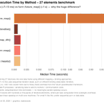
ALT Chart: R zip metadata extraction benchmark on 27 archives. Sequential (lapply/purrr) in ms; furrr parallel ~1s (100× slower). Shows parallelism overhead on small jobs."


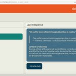
ALT This visual illustrates how a user query (via R) is processed through a local document retriever powered by Ollama. The retriever accesses locally stored documents, which are then passed to a hosted Large Language Model (LLM) to generate a context-aware response. The flow emphasizes privacy, relevance, and control by keeping all data local. Graphics:dataRecode